Introduction
Circulating tumor DNA (ctDNA) refers to fragmented tumor-derived DNA shed into the bloodstream, offering a minimally invasive biomarker for cancer detection, treatment monitoring, and relapse surveillance. Many oncology labs see inconsistent detection results not from gaps in biological understanding, but from pre-analytical variables throughout the workflow that quietly undermine sensitivity. Research shows that ctDNA can range from below 1% of total cfDNA in early-stage cancer to upwards of 90% in late-stage disease, making low-burden detection the most technically demanding scenario.
Digital droplet PCR (ddPCR) is widely recognized for ctDNA detection, achieving variant allele frequency (VAF) detection down to 0.1% in a single well — a full order of magnitude better than the 1% VAF threshold for qPCR. This sensitivity advantage is only realized when sample handling, assay design, input DNA quality, and instrument settings are carefully controlled.
Most failed ctDNA ddPCR experiments trace back to steps upstream of the instrument: wrong tube types, delayed plasma processing, or poor cfDNA extraction — long before the first droplet is generated.
What follows covers the complete workflow: step-by-step sample preparation, quality control checkpoints, assay setup, and troubleshooting. You'll also find guidance on when ddPCR is the right tool for ctDNA analysis versus NGS or qPCR, and which pre-analytical mistakes undermine even well-designed assays.
Key Takeaways
- ctDNA detection by ddPCR relies on absolute quantification of rare mutant alleles in cell-free DNA extracted from blood plasma, enabling mutation tracking without standard curves
- Optimised ddPCR assays achieve 0.01–0.1% VAF sensitivity, making them ideal for minimal residual disease (MRD) monitoring and low-burden disease surveillance
- Pre-analytical errors (wrong tube, delayed centrifugation, poor extraction yield) are the most overlooked failure points — and the first place ctDNA is lost
- Assay success hinges on primer/probe specificity, ≥10,000 droplets per well, optimised annealing temperature, and consistent threshold placement
- ddPCR excels for tracking known mutations in longitudinal monitoring; NGS-based panels are better for mutation discovery or multi-gene profiling
Step-by-Step: How to Detect ctDNA Using ddPCR
Step 1: Blood Collection and Pre-Analytical Sample Processing
Use cell-free DNA blood collection tubes — either standard K3EDTA or specialized cfDNA preservation tubes like Streck Cell-Free DNA BCT. Standard EDTA tubes maintain cfDNA stability for up to 24 hours at room temperature, but processing within 2–4 hours is ideal to prevent white blood cell lysis and genomic DNA contamination. Streck BCT and PAXgene ccfDNA tubes extend stability to at least one week, making them the right choice when same-day processing cannot be guaranteed.
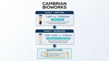
Two-step centrifugation protocol:
- First spin — 1,600 x g for 10 minutes to remove cells
- Second spin — 3,000–16,000 x g for 10 minutes to remove platelets and debris
Research confirms that a moderate second spin at 3,000 x g delivers cfDNA yields comparable to higher-speed protocols at 14,000 x g. The volume of plasma collected — typically 1–4 mL — directly impacts ctDNA yield, as ctDNA concentration is measured in copies per mL of plasma.
Critical pre-analytical rule: Use plasma, never serum. The ctDNA fraction in plasma is significantly higher than in serum because clotting releases genomic DNA from white blood cells, diluting the tumor signal.
Step 2: cfDNA Extraction and Quality Assessment
Once plasma is isolated, cfDNA extraction requires specialized protocols distinct from standard genomic DNA extraction. ctDNA fragments are short — predominantly ~166–167 bp, corresponding to nucleosome-wrapped DNA — and circulate at very low concentrations. Any yield loss here directly translates to missed ctDNA copies downstream.
Extraction chemistry matters: Magnetic bead-based methods are the industry standard for cfDNA workflows. A comparative study of six commercial kits showed median yields ranging from 3.0 to 13.0 ng/mL — up to 4.3-fold variation, with inter-run CVs between 11.8% and 34.6%. Manual spin-column kits often deliver the highest yields, but reproducibility suffers at scale.
Automated bead-based systems like Cambrian Bioworks' Manta (CE-IVD certified) standardize the workflow, reduce hands-on time to minutes, and minimize inter-run variability — especially in clinical MRD monitoring. Manta completes cfDNA extraction in approximately 55 minutes and processes 1–32 samples per run without batching pressure.
Quality assessment requirements:
- Quantify cfDNA using fluorometric methods (e.g., Qubit) — avoid UV spectrophotometry, which overestimates due to contaminating proteins
- Assess fragment size via Bioanalyzer or TapeStation — flag samples with high molecular weight peaks (>1 kb) as contaminated with genomic DNA from lysed leukocytes
- Calculate genome equivalents (GEs): At 3.3 pg per haploid genome, 10 ng cfDNA = ~3,000 GEs; 30 ng = ~9,000 GEs
Minimum input requirements: Most ddPCR ctDNA assays require 1–20 ng cfDNA per reaction. Bio-Rad validates PrimePCR assays at approximately 40,000 GE per 20 µL reaction, but clinical samples often yield far less. Too little input increases false-negative risk, as the number of interrogated GEs sets the statistical floor for rare-event detection.
Step 3: ddPCR Assay Design and Reaction Setup
ddPCR for ctDNA requires mutation-specific TaqMan assays with dual-labelled probes:
- FAM-labelled probe — detects the mutant allele
- HEX/VIC-labelled probe — detects the wild-type allele
Probe design must discriminate single-nucleotide variants (SNVs) or small indels against a large excess (often 99.9%+) of wild-type background DNA. Bio-Rad's PrimePCR ddPCR Mutation Detection Assays are wet-lab validated at 0.1% mutant DNA in wild-type background, and multi-well replication can push sensitivity to 0.005–0.1%.
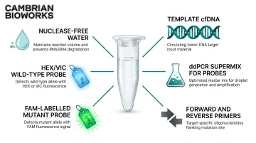
Reaction setup components:
- Template cfDNA (1–20 ng)
- ddPCR Supermix for Probes (No dUTP) — optimised for rare target amplification
- Forward and reverse primers
- Dual-labelled probes (FAM for mutant, HEX/VIC for wild-type)
- Nuclease-free water
Required controls:
- No-template control (NTC) — identifies environmental contamination
- Wild-type-only control (minimum three per experiment) — defines baseline false-positive rate and anchors threshold placement
- Mutation-positive control — verifies expected cluster position and assay performance
Step 4: Droplet Generation, Thermal Cycling, and Data Acquisition
Droplet generation: The reaction mix is partitioned into approximately 20,000 nanolitre-sized water-in-oil droplets, each acting as an independent PCR reaction. Wells with fewer than 10,000 accepted droplets receive a "No Call" from QuantaSoft software — this is a hard quality floor because Poisson-based quantification becomes unreliable below this threshold.
Thermal cycling conditions:
- Hot-start denaturation: 95°C for 5–10 minutes
- 40 cycles (do not exceed 50)
- Annealing/extension: optimise across a gradient (typically 55–65°C)
- Ramp rate: 2.5°C/sec to ensure uniform droplet heating
Optimal annealing temperature is the one that maximises fluorescence amplitude separation between positive and negative clusters while minimising rain. For difficult templates, raising denaturation temperature to 96°C for the first five cycles can improve performance.
Post-PCR droplet reading: The instrument measures FAM and HEX fluorescence amplitude per droplet, classifying each as positive or negative. Absolute copy number is calculated using Poisson statistics: copies per droplet = –ln(1 – p), where p = fraction of positive droplets. No standard curve is needed.
Key Parameters That Affect ctDNA ddPCR Results
ddPCR sensitivity and specificity for ctDNA are not solely instrument-dependent. Four controllable variables determine whether a low-VAF variant is reliably detected or missed.
Input DNA Amount and Genome Equivalent Coverage
The number of genome equivalents loaded per reaction sets the statistical floor for detection. Bio-Rad's "Rule of Three" states: to reach 95% confidence that a sample frequency is 1 in 1,000, you need to identify at least 3 in 3,000 events. This means detecting 0.1% VAF with 95% confidence requires interrogating at least 3,000 GEs.
Practical constraint: At 1,000 GEs (~3.3 ng haploid DNA), a variant at 0.1% VAF appears in just 1 droplet, making replicate reactions essential. Many clinical cfDNA samples yield only 10–30 ng total (equivalent to 3,000–9,000 GEs), which directly constrains the achievable limit of detection (LOD).
Every upstream step that reduces cfDNA recovery raises the minimum detectable VAF. Poor extraction yield, delayed processing, and freeze-thaw damage all compound this effect.
Droplet Generation Quality
Incomplete emulsification or PCR inhibitors produce rain: intermediate-fluorescence droplets that blur the separation between positive and negative populations. Rain arises from biased amplification, fragmented DNA, local secondary structures, and inhibitors. It directly reduces assay sensitivity by creating ambiguous droplets that may be misclassified.
How to assess rain: Inspect 2D amplitude plots. Properly optimised assays show tight positive and negative clusters with minimal intermediate events. If rain is excessive, re-run with:
- Higher annealing temperature (increase by 2–4°C)
- Diluted DNA template (reduces inhibitor concentration)
- Fresh cfDNA extraction (if integrity is suspect)
Annealing Temperature and Probe Specificity
Suboptimal annealing temperature is the primary cause of false positives in ctDNA ddPCR. At lower temperatures, wild-type DNA can partially bind mutant probes, generating spurious signal. Run newly designed assays across a thermal gradient (e.g., 55–65°C) to identify the temperature that maximises cluster separation while avoiding nonspecific amplification.
Validation step: Run a wild-type-only control at your chosen annealing temperature. If mutant-positive droplets appear, raise the temperature by 2–4°C and re-test.
Threshold Placement for Positive/Negative Classification
Thresholds are manually or algorithmically set between negative and positive droplet populations. Inconsistent threshold placement — especially when rain is present — leads to measurable inter-operator variability.
Best practices:
- Draw thresholds above NTC noise levels
- Use wild-type-only controls to anchor the negative population
- Include synthetic mutant standards at known VAF to verify expected cluster positions
- Apply automated threshold algorithms where available
In well-optimised assays, concentration output is not significantly affected by threshold position because clusters are clearly separated. If threshold placement is subjective, the assay needs re-optimisation.
When to Use ddPCR for ctDNA Detection (and When Not To)
ddPCR is not always the optimal method for ctDNA analysis. The right choice depends on the clinical or research question, available mutation information, and required sensitivity.
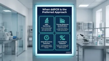
ddPCR is the preferred approach for:
- Monitoring known somatic mutations for MRD after curative treatment
- Quantifying ctDNA burden during therapy to assess treatment response
- Detecting recurrence at low tumor fractions before imaging or clinical symptoms appear
- Validating liquid biopsy findings from NGS or other platforms
A landmark study of 851 stage II-III colorectal cancer patients demonstrated that serial dPCR ctDNA detection was prognostic of recurrence with HR = 30.7 (95% CI 20.2–46.7, P < 0.001), with 87% cumulative ctDNA detection in patients who recurred. In breast cancer, ddPCR-based mutation detection preceded clinical detection of metastasis in 86% of patients.
Choose alternatives instead when:
- Mutation landscape is unknown — use NGS-based ctDNA panels for mutation discovery
- Multi-gene profiling is needed — NGS provides broader genomic coverage
- VAF is expected to be high (>1%) and cost is a constraint — qPCR is cheaper
- Tumor-informed approach is not feasible — use untargeted liquid biopsy methods
Each method involves a real trade-off between cost, speed, and discovery power:
| Method | Strength | Limitation |
|---|---|---|
| ddPCR | 5–8.5× lower cost than NGS; same-day turnaround | Requires prior knowledge of mutation target |
| NGS | Broad genomic coverage; enables mutation discovery | Higher cost; longer analysis times |
| qPCR | Lowest cost per reaction | Insufficient sensitivity for MRD-level detection |
Common Mistakes and How to Troubleshoot Them
Pre-Analytical Errors
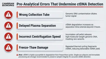
The majority of failed or unreliable ctDNA ddPCR experiments trace to pre-analytical errors:
- Wrong collection tube (serum instead of plasma, or non-preservative EDTA with delayed processing)
- Delayed plasma separation beyond 24 hours in EDTA
- Incorrect centrifugation speed (insufficient removal of cellular debris)
- Using frozen-thawed plasma without validating fragment integrity
Plasma subjected to three freeze-thaw cycles exhibits significant cfDNA degradation, reducing the ratio of longer to shorter fragments. These errors inflate genomic DNA contamination and degrade ctDNA yield before the assay even starts.
False Positives From Wild-Type DNA Amplification
False positives typically stem from a suboptimal annealing temperature or probe cross-reactivity. To confirm, run a wild-type-only control under identical conditions — if mutant-positive droplets appear, the signal is artifact. Increase annealing temperature by 2–4°C and validate against both wild-type and mutant controls before proceeding.
Insufficient Droplet Count Per Well
Likely causes:
- Contaminants in DNA eluate (residual salts, alcohol carryover from extraction)
- Oil quality issues (expired Droplet Generation Oil or gaskets)
- Pipetting errors (bubbles introduced into cartridge wells)
- Exceeding maximum DNA load (>66 ng/well for undigested DNA)
Fix: Re-extract or dilute sample, check oil cartridge expiration dates, verify pipette calibration, and review cartridge assembly.
Threshold-Setting Inconsistency Across Operators or Runs
Threshold placement is one of the most operator-dependent steps in ddPCR. To reduce run-to-run variability:
- Use synthetic mutant standards at known VAF as consistent positive controls
- Include no-template controls (NTCs) in every run
- Apply automated threshold algorithms where available
- Document threshold placement in SOPs and enforce the same logic across experiments
When these controls are built into every run, inter-run comparisons become far more defensible — especially in longitudinal monitoring where small VAF shifts carry clinical weight.
Conclusion
ctDNA detection by ddPCR is a powerful but precision-dependent workflow. Its sensitivity advantage over qPCR — reliably detecting VAFs of 0.1% or lower — is only realised when pre-analytical variables, input DNA quality, assay design, and threshold settings are all carefully controlled.
Most failures originate upstream of the instrument. Wrong tube type, delayed processing, poor extraction yield, or contaminated samples sabotage even the best-designed ddPCR assays before the first droplet is generated.
Standardisation of these early steps — through validated protocols, automated extraction platforms like Cambrian Bioworks' Manta, and rigorous pre-analytical quality control — is as important as the ddPCR run itself.
When executed correctly, ddPCR-based ctDNA monitoring delivers clinically actionable MRD surveillance data, enabling recurrence detection weeks to months before imaging or clinical symptoms appear. That means treating pre-analytical quality control with the same rigour you apply to the instrument run — because sensitivity lost upstream cannot be recovered at the detector.
Frequently Asked Questions
What is dPCR and ddPCR?
Digital PCR (dPCR) is a method that partitions a sample into thousands of individual PCR reactions to enable absolute quantification without a standard curve. Droplet digital PCR (ddPCR) is the most widely adopted format, using water-in-oil emulsion to generate approximately 20,000 droplet partitions per reaction, each read individually for endpoint fluorescence.
When is ddPCR better than qPCR?
ddPCR outperforms qPCR when detecting rare variants at very low allele frequencies (below 1%), as in ctDNA monitoring. It achieves 0.1% VAF detection versus 1% for qPCR, as it does not rely on a standard curve and is less affected by PCR efficiency differences. This makes it the preferred tool for MRD detection and low-burden disease surveillance.
What is ctDNA and how is it different from cfDNA?
Cell-free DNA (cfDNA) refers to all fragmented DNA circulating in plasma from any cell type, while ctDNA is the tumour-derived subset of cfDNA. ctDNA typically constitutes a small fraction of total cfDNA and carries tumour-specific somatic mutations that distinguish it from normal cfDNA, enabling its use as a cancer biomarker.
What sample type is best for ctDNA detection by ddPCR?
Plasma from peripheral blood is the standard sample type, collected in specialised cfDNA preservation tubes or processed rapidly (within 24 hours) in EDTA tubes. Serum is not recommended due to genomic DNA contamination from clotting. In standard EDTA tubes, processing delays beyond 4 hours can similarly compromise sample quality.
What is the lowest variant allele frequency ddPCR can reliably detect?
Optimised ddPCR assays can detect VAFs as low as 0.01–0.1%, depending on input DNA amount, assay design, and background noise. Reaching 0.1% VAF at 95% confidence requires ≥3,000 genome equivalents, optimised probes, and careful threshold placement.
Can ddPCR be used for MRD monitoring in cancer patients?
Yes. ddPCR is increasingly used for ctDNA-based MRD monitoring post-treatment, detecting residual tumour DNA weeks to months before clinical or imaging-based recurrence — provided the patient's specific somatic mutation target has been identified from the primary tumour or baseline liquid biopsy.